PCA ICA course

I'm also finally done teaching the PCA/ICA course in the student comp class. I really like how serious the class is, I guess classes are a lot better when you have all the best kids and their motivated -- and also you aren't really responsible. I really enjoyed it, because it forced me to learn ICA pretty hard. And now I feel a lot more confident about it, and i will seriously be able to do some stuff with my data with ICA.

I like a lot of the ideas in the homework, but it definitely can be better. Honestly it is pretty easy right now, but some parts are confusing. But I really enjoyed people's answers and i thought that it was tricky in the right ways. It made me happy to see their answers. 

The ICA part was hard because I was a jerk and did it in python, and the mac kids had problems. But, I think its a really good exercise and theres a lot more to explore. I had them just add noise and see what happened, and i made algorithms to match up the ICs and print out the cost. i wanted them to come up with some more things, but nothing too fancy. They could also change the mixing matrix such that they had more or less microphones to actually see what happens.

I realize now that I had no idea how to use fastica for the image analysis. The problem was that it is not like PCA at all, and I just assumed that it was. It is interesting because the ICs are scalar-invariant. So they come out in no particular order and there's nothing that says how important they are -- there are no eigenvalues. I don't quite understand why they don't get sorted by whatever it is they're optimizing -- their non-gaussianity. Fastica is supposedly doing some optimization, so why don't each of the components have an optimization value, can't you sort by that?

The other useful thing would be to find the mixing matrix. It wouldn't really be that hard -- its basically fitting the microphones with the ICs, but maybe there are better and worse ways... I just did a linear regression to see which ICs matched up with the original components. I guess if you just matched them to the data, wouldn't it come out to an exact mixing matrix? 

Yi Zuo

Hosted Yi Zuo this week. She was the seminar speaker and talked about how dendritic spines form during learning tasks. I took away a few extra things from her talk -- one was that the spines stopped forming as much once the behavior had plateaued, kinda like perceptron learning rule (once you get it right stop changing). The other was that spine growth was present shortly after training, but there was no spine elimination. But, this was only true if the imaging was done immediately after -- imaging a day after then there was increased spine elimination to compensate for the growth. It just has to be something to do with sleep.

I actually had a really good time talking with her and learning about her life. I was very worried because she was quite Chinese and I was afraid it was going to be hard to communicate. But she was very talkative, maybe even too talkative, but I was happy because not too many awkward silences. I couldn't believe how energetic she was in general. I was exhausted and I was doing nothing for most of the day, she had talked to so many people: Mayford, Jim Connor, Lunch (Jeremy Biane, Tom Gillespie, ...), Zheng, Scanziani, Komiyama, the talk, dinner (andy, sam, adam, jeremy, heidi, kathleen). And then jeremy gave her a laptop talk about his data. Damn she was a trooper.

Functional mapping of single spines in cortical neurons in vivo

Chen, X., Leischner, U., Rochefort, N.L., Nelken, I., Konnerth, A. (2011). Functional mapping of single spines in cortical neurons in vivo. Nature 475.

Two-photon (LOTUS) imaging of individual spines in auditory cortex. Present tone stimuli at different frequencies and volumes. Spines show a variety of tuning properties, but no clear clustering on dendrites is observed.

Figure 3 | Frequency tuning and heterogeneous distribution of individual
active spines. a,Upper panel: two-photonimage of a dendritic segment of a layer
2/3 neuron (average of 6,250 frames). Lower panel: calciumresponses (average of
five trials) from two spines (S) marked by red arrowheads in the upper panel,
during 11 pure tones (from 2kHz to 40 kHz at 0 dB attenuation). Two
neighbouring spines indicated by blue arrowheads did not respond to any of the
11pure tones.b,Upper panel: frequency tuning curve of thenarrowly tuned spine
S1 shown in a. Data points are the mean values of response amplitudes from
five trials. Lower panel: average tuning curve normalized to the highestamplitude
(n538 spines, 10 neurons). c,Upper panel: frequency tuning curve of thewidelytuned
spine S2 shown in a. Lower panel: average tuning curve, normalized to the
highest amplitude (n546 spines, 10 neurons). Error bars in b and c show s.e.m.
d, Distribution of frequency tuning widths (DFrequency) of pure-tone-activated
spines (n584 spines, 10 neurons). e, Heterogeneous distribution of pure-toneactivated
spines along dendrites. Cartoons of dendritic segments from four
neurons, with numbers indicating the effective frequencies for each active spine.
Narrowly tuned and widely tuned spines are indicated by red and blue dots,
respectively. The neurons correspond to, respectively, neuron 25, neuron 27,
neuron 29 and neuron 30 in Supplementary Table 1. f, Plot of the most effective
frequency of a given spine versus themost effective frequency of its nearest active
spine (seeMethods).Dots along the red line correspond to pairs of spines that had
the same most-effective frequency (n569 pairs, 24 dendrites, 10neurons).
g, Plot of the distance between neighbouring active spines versus the difference
between their respective most-effective frequencies. For each pair of spines, the
reference spine (blue circle) was defined as the left spine and the test spine (red
circle) was defined as the neighbouring active spine on the right. The
measurements were performed sequentially from left to right in each dendrite
(n551 pairs, 24 dendrites, 10 neurons). Dots along the red line correspond to
spine pairs that had the same most-effective frequency. Numbers on the right
indicate distance ranges between pairs of spines with a difference between their
most effective frequencies of 0–1, 1–2, 2–3 and 3–4 octaves.

ICA

The motivation behind developing ICA can be illustrated by a classic problem -- the "Cocktail Party" problem. The basic idea is that you are at a big party and you hear the voices of many different people talking. Your ears are picking up the sum of all of these people's voices and your brain has the task of separating out each of the voices. Each ear receives a slightly different signal -- say your left ear is closer to speaker 1, and the other ear is closer to speaker 2. The left ear would receive a stronger signal from speaker 1 and a weaker signal from speaker 2. Mathematically each ear is just receiving a weighted sum of all of the signals.

x = M*s

So x is what your ears pick up, s are the speakers at the party, and M describes how the signals from each of the speakers get mixed together to make the observed signal. This is the "Mixing Matrix".

The assumptions about the problem that we are trying to solve is that the signals that we observe are actually mixtures of signals that are independent -- the speakers talking at the party are not influencing each other. So how do we pull out the independent signals from the observed data in x? What exactly do we mean by independence?

There are some strict probabilistic definitions of independence -- namely p(a,b) = p(a)*p(b). These p's describe the full probability distributions of the signals, and independence means that the chance of observing a and b together is equal to the product of observing each of them independently. If this holds true across the entire probability distribution, then the signals are independent. However, this definition is almost useless for any realistic application, because it would require accurately estimating the complete distributions and the complete joint distribution of the inputs. 

Correlation is something that you could easily calculate practically, but no correlation does not necessarily imply independence. Independence, however, does imply that no correlation. A sine wave and a cosine wave plotted against each other would create a circle -- data in the shape of a circle would clearly be uncorrelated. However, these data are obviously not independent.

A big intuition about how to determine independence comes from the Central Limit Theorem. This is one of the most fundamental ideas in probability and statistics. The central limit theorem states that the summation of many independent random events will converge towards a gaussian. It doesn't matter what the probability distribution of the individual events are -- they can be uniform, binary etc, but adding many independent elements together will produce a Normal distribution. A nice example is rolling dice. If you roll one die, then there is a uniform probability that it will land on one of the numbers 1-6. If you roll two die, then the sum of the die no longer has a uniform probability -- the sum is most likely to be 7, and least likely to be 2 or 12. As you add more and more dice the probability distribution gets closer and closer to looking like a bell curve -- a Normal/Gaussian distribution. The Central Limit Theorem is why a Normal distribution is called Normal -- we see these distributions all over the place in the real world because independent events when summed together take this shape. 

For ICA we are assuming that several independent components are being mixed together to create our observed signals. The Central Limit Theorem states that if we mix independent components then we get something that is more Normal than the original components. Thus the goal of ICA is to find a projection of the mixed signals that is the LEAST Gaussian or the most non-gaussian. ICA thus becomes an optimization problem where we are trying to find a projection of the data that gives us the most non-gaussian components.

In order to solve the optimization problem, we must define what we mean by non-gaussian -- how do we measure non-gaussianity? There are several possible ways to estimate the gaussianity of data, and each have different trade-offs. Estimators can be optimal but require a lot of data or they can be efficient but biased. The field is not fully set on the "best" way of estimating non-gaussianity, but there are a few ways of doing it which stem from probability theory and information theory. In reality these different metrics are actually quite similar, and probability theory and information theory are actually mathematically linked -- several studies have shown how estimators derived from probability theory are actually identical to some estimators derived through information theory. There is in fact an underlying mathematical structure that links both fields.

One of the most prominent and conceptually simple ways of measuring non-gaussianity is to use the "Kurtosis". The kurtosis is related the 4th order moment of a probability distribution (the first is the mean, the second is the variance, the 3rd is known as skewness). The kurtosis is the peakiness of the distribution. There are infinitely more moments, and all are defined by raising the expected data to different powers (the nth moment is E(x^n), where E is the Expectation operator). Kurtosis is technically the "excess" of the 4th moment, and is usually compared to the Kurtosis of a Gaussian distribution. A Gaussian distribution has a 4th moment of 3-sigma^4 (where sigma is std). The kurtosis is defined relative to a Normal distribution with variance of 1, and so you just subtract out the kurtosis of a Normal distribution with the same variance as the data -- K = E(x^4) - 3. 

ICA

I'm teaching ICA in the comp-neuro student course and I'm studying up on it today. I'm just going to try and make an outline of the important points to cover. This tutorial is really good, and will serve as the basis.

Here are the main points I want to cover:

1. Motivation
1. The cocktail party problem
2. Definition -- matrices and data
3. Ambiguities
4. Illustration
2. What is independence?
1. Central limit theorm
2. Nongaussian is independent
3. Estimators of nongaussianity
1. Kurtosis
2. Negentropy
3. Others
3. Preprocessing for ICA
1. Centering
2. Whitening
3. PCA
4. Fast ICA
5. Neuroscience Applications
1. EEG
2. Imaging

Nonlinear Population Codes

Shamir, M., Sompolinsky, H. (2004) Nonlinear Population Codes. Neural Computation 16: 1105-1136.

Not exactly what I thought this was about. They are crafting a population code such that they can vary the noise correlations of the neurons, something they argue is biologically relevant. This sets up more information about the stimulus in the higher-order statistics of the firing rates -- i.e. there's more information if you look at the covariances than just at the mean.

So they make a 2-layer FF neural network that has a quadratic non-linearity in the hidden layer. Then they can apparently get the stimulus information much more close to optimal through the network. This quadratic non-linearity is important for conveying the information in the second-order statistics, and some how decorrelates the neural signals. This makes the standard linear readout in the output layer the same as the typically way of reading out population codes.

So maybe worth mentioning something like -- non-linearities in neuron's IO functions could be important for extracting information from the higher-order statistics of neuronal firing (Shamir & Sompolinksy, 2004) or matching the statistics of the input probability distribution (cite needed). I remember some paper, I think we read it in Tanya's course, that discussed the idea that a sigmoid non-linearity is informationally optimal if the input has some Gaussian distribution. The most probable events are in the middle of the Gaussian, which is the steepest part of the sigmoid, and the steeper the output the more information about the input is available.

Noise and Shunting

Ulrich, 2003; (noise)
Dynamic clamp in L5 pyr somatosensory cortex. Shunting multiplies the voltage, but not the spiking. He adds a GABA blocker and shows that it has an additive effect.

Chance, Abbott, Reyes 2002; (noise)
Dynamic clamp of rat somatosensory cortex slices L5 pyr. Random incoming excitatory and inhibitory synaptic inputs, increasing the "rates" of the inputs causes more shunting and more variance in the injected current. They inject driving current on top of the noisy current, more noise means the gain is decreased. Shunting inhibition without noise leads to shift in the firing-rate curve. They make a model, but its not a simulation -- they have an analytic description of firing rate from noise. The gain effect in the model goes away for high firing rates. Background excitation and inhibition must be balanced.

Mitchell & Silver, 2003; (noise)
Dynamic clamp of cerebellar granule cells. If synaptic excitation is frequency dependent then you get the gain effect, step currents give additive effect. Their IF model gets step shunting inhibition and synaptic excitation, and shows a gain and offset effect. The gain effect requires that the variance of the excitation increases with the level of excitation.

Capaday 2002; (inh feedback or neuromodulators)
Two compartment HH-like conductance model of motorneuron (dendrite and soma). He concludes that the mixture of excitatory and inhibitory conductances do not matter for gain, its not synaptic currents per se, but ligand action on receptors capable of activating intrinsic conductances. Inhibitory feedback can also be used to produce gain (circuit mechanism).

Gabbiani & Knopfel 1994;
Granule cell model -- multi-compartment, but "compact" (which effectively makes it a single compartment, I guess they just have a very low intra-cellular resistance). Shunting inhibition is additive and not multiplicative. This is just Holt & Koch before they described it.

Doiron et al. 2000; (noise)
Complex conductance model of pyramidal cell in electric fish and LIF model. Subthreshold shunting is divisive, in spiking regime additive. They get gain but only if there is stochasticity in the inhibition, and only for low firing rates. The gain is only there if the variance of the inhibition increases with the mean conductance.

Abbott & Chance 2005;
"(It is important to note that, despite comments in the literature to the contrary, divisive inhibition
of neuronal responses cannot arise from so called shunting inhibition. As has been shown both theoretically (Gabbiani et al., 1994; Holt and Koch, 1997) and experimentally (Chance et al., 2002),"
Review based on Chance 2002. They both can suggest that the circuit is doing a driving and balancing act to produce the gain, but require changes in the noise variance.

Salinas & Abbot 1996; (circuit)
Recurrent network for gain control.

Hahnloser et al, 2000; (circuit)
Analog circuit, feedback recurrent excitation and inhibition sets up a gain modulation. Can change the inhibition and alter the gain.

Ayaz & Chance 2009; (noise, circuit)
Normalization pool and modulatory pool, normalization pool driven by the stimuli within RF, modulatory pool driven by stimuli in surround. Inhibtion increases proportionally to the sum of both pools. When the pools increase noisy synaptic input you get a gain effect.

Prescott & De Koninck 2003; (noise, dendritic saturation)
Similar to Chance 2002, need noise but also dendritic saturation apparently helps. Multi-compartmental model of L5 pyramidal cell. Many of the other papers talked about how the gain effect goes away for higher inputs, the saturation prevents that.

Burkitt, Meffin, Graydin 2003; (noise, circuit)
LIF model. Two regimes: linear - excitation and extra leak from background noise cancel out, non-linear - leakiness dominates resulting in diminished gain.

Seeing White: Qualia in the Context of Decoding Population Codes

Lehky, SR. Sejnowski, TJ. (1999) Seeing White: Qualia in the Context of Decoding Population Codes. Neural Computation 11: 1261-1280.

So they argue a very interesting point: in the context of color vision, the typical decoding methods pick out a single value. But when you see white you are seeing the combination of several wavelengths, and the color you experience is separate from the individual wavelengths. Essentially this generalizes to mixtures of stimuli, where typically population codes account for only a single stimulus value. Complex stimuli are represented in a different way than just their average or maximum likelihood estimate, even a multi-modal estimate may not be correct.

White can be thought of as an arbitrary symbol or label marking the presence of a certain combination of color-tuning curve activities. Decoding is not specifying a single physical parameter, but to specifying some region in an abstract psychological space. There is a straight-forward linear transformation from wavelength space (or cone activation space) to 2D CIE color space (which is like HSV). (The mapping actually requires division to compute). Brightness is the 3rd dimension and is represented by absolute levels of activity -- gray and white map to same CIE point, but differ in brightness.

They make a 4 layer NN to get from cones to CIE. Layer 2 is color opponent units "+r-g" which are similar to RGCs. Layer 3 is noncolor opponent and they make a comparison to neurons in V4, this was just the hidden layer of the network.

This, in a way, is just mapping from one population-code space (wavelengths) to another space (CIE color). This is a symbolic representation of a set of variables, which is likely more behaviorally useful (thus is why this system evolved).

Arthur Konnerth

Arthur Konnerth is the seminar speaker this week. We had a nice talk at lunch about how electro-physiology was bullshit because of how it interrupts the normal circuit properties of the cell. Stabbing into the cell ruduces the membrane resistance adds a time constant. He was quite challenging no matter which way the conversation went, it was an interesting way of talking about science. At times I felt like I would make a statement agreeing with his point and in return he would come back and question its validity. A prime example was how it would be great to measure the absolute voltages of a cell. I agreed, and then he came back at me questioning the need to. A lot of talk about what it is we are trying to do, and he really challenged me on what I think would come of mapping efforts. We hit upon exploratory vs. hypothesis driven types of Science.

He gave a good talk. It was mainly about the paper where he could measure the individual spine calcium signals and showed that the "inputs" to the dendrites -- calcium in spines, were tuned like "salt and pepper" across the dendrites. Some bias with the neuron's receptive field, but he said he didn't really have enough data to prove so. It was nice he showed that even across different cortical areas there was this salt and pepper to the inputs. (Mainly looking at L2/3 pyramids).

Visualization of image data from cells to organisms

Walter, T. Shattuck, DW. Baldock, R. Bastin, ME. Carpenter, AE. Duce, S. Ellenberg, J. Fraser, A. Hamilton, N. Pieper, S. Ragan, MA. Schneider, JE. Tomancak, P. Heriche, JK. (2010) Visualization of image data from cells to organisms. Nature Methods 7(3)

Lots of data is a problem, need tools to visualize it all, put it all together etc. There are many technical challenges -- file formats, meta-data, etc.

You can use color coding to represent higher-dimensional data, but that only gets you to 5-6 dimensions. Some people have considered converting data to sounds "to take advantage of people's ability to distinguish subtle variations in sounds patterns." (‘data sonification’ (T. Hermann,T. Nattkemper, H. Ritter and W. Schubert. Proc. Mathematical and Engineering Techniques in Medical and Biological Sciences, 745–75))

DTI - several ways of visualizing the tensor directions, gives you 3D data set where each voxel is essentially a 3D value (the colors actualy can work here.)

Registration: simplest form is designate one acquisition as the reference and registering all others to it, but introduces a reference-specific bias. Atlas registration registers to an idealized expert-definied atlas. Something like SIFT might be useful. And here's a paper about gene expression atlases.

I got a bunch of other registration papers, and visualization tool papers from this review to look over.

Cell identification is a sub-problem of vision

The computational challenge of this project is that in many ways identifying cells is a vision/pattern recognition problem. Essentially the visual system is collecting information about the world, creating categorical features from that information, and then using low-level categorizations to make features for the next level up. Its obviously doing a lot more than just these things, but at a basic level this is what powers the visual system.

The most basic features are something like edges/gabor filters. These features can be recreated from algorithms such as ICA, or sparse coding of the visual world. The visual system balances a representation that is complete (or even over-complete) with a representation that is efficient. The representation must be complete (especially at the lower levels), because it isn't like you could be shown something and not see it. Somehow the information is being represented no matter what is being shown, which implies that all information has a representation of some sorts. Efficiency is related to the dimensionality of the representation, and in of itself has important computational properties. An efficient representation transmits only the needed information to understand what is happening. If one could build a model that has a low-dimensional parameter space, then one could only need to transmit the low-dimensional information of those parameters. This would be highly efficient.

What's remarkable is that the visual system is likely able to make these dimensionality trade-offs. When a stimulus that is familiar and has a well-developed low-dimensional parameter space, it is likely only activating a few neurons (but perhaps very strongly). Each of the neurons is acting as a vector in some high-dimensional space, and when only a few need to be activated, then only a low-dimensional subspace is being used for representation. When a strange stimulus, or one that has no low-dimensional description (i.e. white noise), appears then the visual system uses more neurons to represent all the information. It has to since it has to be complete. The learning in the brain is essentially trying to take the high-dimensional representations of unlearned stimuli and find a low-dimensional "model" that also represent the information.

My project is in a way doing a simple vision task. We're skipping some of the stages by developing useful features manually, and then building a good, high-dimensional representation of the properties of the cells. The idea I'm trying to build for the identification of cells is just one stage of the visual algorithm. The challenge is to take the feature space and then start to make classifications on the data. The hierarchy is important, because it allows you to simultaneously represent the data at different levels. An individual cell, say the N cell, as a representation would be at the top. Then perhaps all of the N cells at the next level, then the T and N cells and maybe the AP. Then eventually you get all the way down to just all cells at the bottom. With the hierarchical design, you automatically categorize the individuality of each cell as well as put all of the cells into clusters and describe the build-up of the features. A person is the combination of hands, arms, face, legs, body etc, a face is a combination of a head, eyes, nose, a mouth, an eye is a black circle surrounded by a colored circle surrounded by white. All of these are all together represented simultaneously in the brain. This builds a oneness by a hierarchical representation, which enables the gestalt along with the specific together. I somehow want to capture this in the classification of cells.

What's useful is that the visual system reorganizes its features (or the low-dimensional representation of the categories at each hierarchical level), based on the features that are somehow more informative. And it can alter those features based on how well they classify. I will be starting with some high-dimensional feature space (it won't even really be that high). The first stage will be some sort of dimensionality reduction that creates an efficient feature space -- this will be important because I can plug in similar features that are just slightly different transforms. So I can use absolute positions, position relative to packet, reflected position, which would be a 6-dimensional feature space (3x2 for x and y), but these are not orthogonal dimensions and will be somewhat redundant, but will together in total contain more information than just the individual feature. A low-dimensional projection of this feature space will remove the redundancy of the features and emphasize the useful information from these slightly different representations. So a truly two-dimensional feature (x,y position) is build from an inefficient 6-dimensional representation that relates the information in different ways, which is then reduced to a lower-dimensional space that is more useful for classification. The final space will be more than just two dimensions, but probably only 3 or 4 would be enough to almost fully capture the different information of the position feature.

It would be cool to just use like anatomical features as a starting point to somehow classify all of the cells. Then just from position and size information, you could find some hierarchical clusters that tries to classify the cells from just anatomy. This would take you a long way to classing all of the cells, but probably couldn't fully classify them all. One class would be like the sensory cells in the lateral packets, another would be the small cells around them, another would be the medium cells an the anterior lateral, etc etc. You probably wouldn't have enough information to fully pull out the N cells from the T cells with just anatomy alone, but just this clustering would be very useful. Once we have the functional data, it would be cool to try and cluster without any of the anatomy, and see if cells fall into functional clusters. All of the functional dimensions could also have these high-dimensional, but reduntant representations to keep as much information as possible -- i.e. the swim oscillators can have 2 dimensions representing the swim relative to DP, relative to other oscillators (i.e. 153), etc.

Algorithms for BRAIN -- Human Connectome Project

The BRAIN Initiative was announced this week, and it has been really exciting for people like me already trying to map a nervous system. I've been trying to figure out what to do over the next year to finish my thesis, and the algorithmic side of this project is really the area that needs the most attention. The big challenge will be to create something that not only helps with my thesis project of mapping the neurons in the leech ganglion, but also provides a useful tool for other large-scale brain mapping projects.

The human connectome project comes to mind as a very similar problem from the algorithmic side. This project is at the macro-scale for connectomics -- attempting to map the connectivity of different brain regions using MRI, fMRI, DTI etc. There are several challenges to overcome from the vast amount of data that is being collected, and the algorithms that will help to solve my problems could also be useful in this context. Everyone understands that getting maps of neural activity will be extremely important in understanding how the brain works, but they don't realize that once you have that data, there is a long way to making any sense of it.

Part of the problem with the human connectome project is the problem of registration. Registration is exactly my thesis project -- identification of all of the pieces. In my case I'm trying to identify individual cells across different animals. In the human connectome project, the challenge is to identify individual brain regions. These regions must be consistent and somehow identifiable across individuals. In the fMRI world, typically a brain is mapped on to the "canonical" brain, which is essentially just some ladies brain. The prominent features are analyzed by humans and these features are used to morph individuals onto a single brain-space. The human connectome project is expanding upon this by adding in all the DTI connections, and some fMRI response data to help identify different brain regions.

The feature abstraction that we have started is going to be a useful way of putting these different data sets in the same space so that registration algorithms can work universally. In HCP they get function and anatomical data as well as connectivity data across different brain regions, but like in the leech the same brain region may not be in exactly the same spot etc. But, across animals the same brain regions should have similar functional properties and similar connectivity profiles. By taking all of these as abstract features and then doing registration analysis on this feature space, there may be a consistent tool that can tackle both of these problems and more.

A way of looking at connectomics is based on graphs, which has an extensive mathematical/theoretical background/tools. Graphs are made up of nodes and edges. The connectome is specifying all of the edges -- which nodes are connected. The challenge is to figure out how many nodes there are, and how to match nodes across different individuals/organisms.

Transfer Function Review

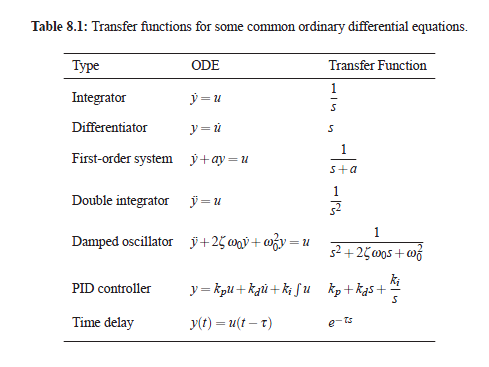
The transfer function of the multiplicative feedback would be really interesting to figure out. Here's Murray's book (he taught the CDS class at Caltech). I was looking through chapter 8 - Transfer Functions to remember how to compute them.

All signals can be represented by a complex exponential - exp(st), s= \sigma + i\omega. Linear systems are represented by two equations, a diff eq and linear eq:

dx/dt = Ax + Bu
y = Cx + Du

where u is the input signal, and y is the output signal. The transfer function is simply the input-output function. For a linear system with where the output is some order derivative (or integral) of the input then the transfer function is just:

G(s) = b(s)/a(s)

Where a(s) and b(s) are polynomials. Poles and zeros are the roots of a(s) and b(s), respectively.

And then you can do "Block Diagram Algebra" for more complex systems.

And this can all be further formalized with laplace transforms, but that's basically what he was doing before.

Do we even need to calculate sqrt?

I've been thinking about this some and in terms of a feedback loop it may not be necessary to do the sqrt part. If the interneurons were doing the L2 norm correctly in a feedback loop, then it should always settle to an equilibrium value where the length of the vector is 1. This will be true no matter how large the inputs are, and it should be the only stable state. But if the sqrt is removed, then the normalization should be over-compensated when the vector length is above 1 and under-compensated when the vector length is below 1. This still sends the dynamics to the same stable state, though, it would just probably over/under shoot, but still settle to the correct length.

Without doing the square summation the feedback normalization was not strong enough, I guess, to compensate for the feedback excitation. I think its just that the feedback doesn't grow enough compared to the excitation, so it cannot keep the population normalized to a single value. But if the feedback grows too much, it would just reduce the activity too much and then it would settle to some eq.

...yeah of course not. I'm actually less sure if its even possible regardless if the sqrt would work -- at least from a purely feedback stance. If there's more FF, then there would have to be more inhibition to compensate, but if it always decayed to a stable integral, then the inhibition level would have to be the same. If the inhibition was the same, it couldn't possibly reduce the interneurons enough. So there can't be a feedback circuit that always maintains a normalized vector -- unless you add in feed-forward inhibition too.

It does a pretty good job of keeping it under control in general. I don't have to fiddle with the knobs too much. The feedback has some interesting properties.